STEPS OF USING MICROSOFT EXCEL

Microsoft Excel is a powerful spreadsheet application that can be used for anything from a simple database all the way up to a full fledged Windows application full with windows forms, macros, and add-ons. You can use Excel to calculate a car loan payment, graph data, manage customer records, keep an address book, etc.
Excel is currently used by most large financial institutions for daily financial data analysis. It has a huge range of financial functions, formulas, and add-ons that allows you to use Excel to store and analyze data in a simple, quick way.
In this tutorial, we’re going to go through the basics of Excel: creating workbooks, using worksheets, entering data, using formulas, etc so that you can become comfortable with the software and begin to learn on your own by playing around with it.

First Steps Into Excel

First, let’s open Excel and take a look at the interface of the program. Open Excel and a new workbook will automatically be created. A Workbook is the top level object in Excel. It contains Worksheets, which hold all the actual data that you will be working with. A workbook starts off with three worksheets, but you can add or delete worksheets at any time as long as there is at least one worksheet in a given workbook.
Now depending on the version of Excel you are using, the following screen may look completely different. Microsoft has changed the interface wildly from Office 2003 to 2007 to 2010 and finally in 2013. Unfortunately, I have to pick a version to write this tutorial in and I’m currently choosing Excel 2010 because it’s right in between 2007 and 2013 and all three versions use the new ribbon interface. Office 2013 just makes the look more clean, but the overall layout is still the same.

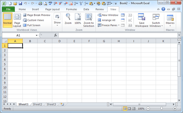
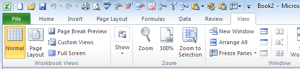
Across the top, you have the Excel ribbon with multiple tabs and also a bunch of little icons at the top in the Quick Access Toolbar. These little icons let you perform very common Excel functions like adding or deleting rows in the worksheet or freezing panes, etc.

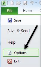
If you want to customize the ribbon interface, i.e., add a button or option that you miss from an older version of Excel, you can do that by clicking on File and then clicking on Options.

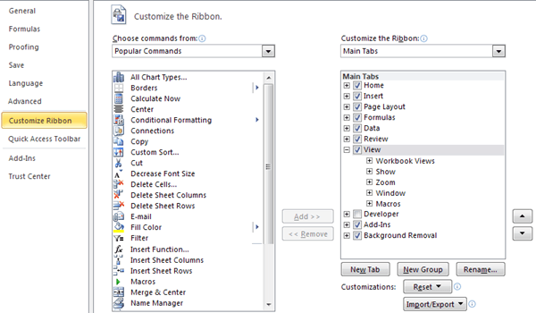
Now click on Customize Ribbon at the bottom left and you’ll be able to add or remove any possible option you could possibly want. By default, it shows you the popular commands, but you can click on the dropdown to see all the possible options for different tabs. Also, one option I really like is choosing Commands Not in the Ribbon from the dropdown. That way you can easily see which commands are already not on the ribbon and then add any you feel you’ll need.

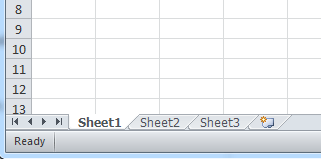
At the bottom of the screen, you’ll see three sheets, named Sheet1, Sheet2, and Sheet3. This is the default number that every Excel workbook starts off with.

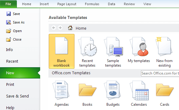
On older versions of Excel the task pane was located on the right side of the screen, however that has now been removed and all the functions have been moved to the File tab. This is where you can perform many common tasks such as opening a workbook, creating a new one, printing and more.

Getting Started with Excel

The best way to learn anything is to actually do something useful and Excel is the best example of this! Let’s say you are a high school or college teacher and you want to keep track of your student’s grades, calculate their average and tell them the lowest grade they would need to get on their final exam in order to pass the class.
Sounds like a simple problem and it is (once you get the formula in your head)! Excel can do this for you very quickly, so let’s see how.
First off, let’s enter some data into the cells in Excel. In Excel, the columns are labeled starting from A and continuing to Z and beyond. A cell is simply a particular row number and column, i.e. A1 is the very first cell in an Excel worksheet.
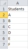
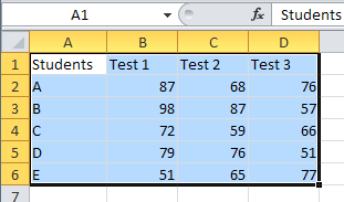
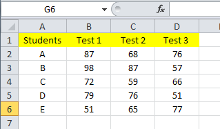
Let’s type Students into well A1 and then type A through E as the student names continuing down column A as shown below:

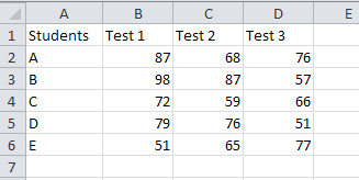
Now let’s enter Test 1, Test 2, and Test 3 into cells B1, C1, and D1 respectively. Now we have a 5×4 grid, so let’s fill out some fake test grades also as shown below:

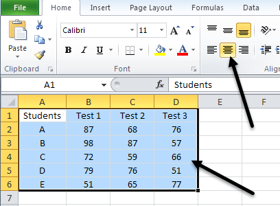
Now let’s learn some of the basics of formatting cells in Excel. Right now our table doesn’t look very nice since the text and numbers are aligned differently and the headers are not visually separate from the data. First, let’s center all the data so that things look nicer. Click on cell A1 and drag your mouse down to cell D6 to highlight the entire data set:

Then click on the Home tab and click on the Center Justify button. The grid is now nicely centered with all the data directly underneath the headings.

Now let’s look more at how we can format Excel cells. Let’s change the color of the first row to something else so that we can clearly separate the header from the data. Click on cell A1 and drag the mouse while holding the button down to cell D1. Right click and select Format Cells.

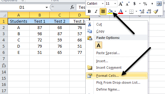
Now there are two options you have at this point. You’ll notice in the image above, a normal right-click menu that starts with Cut, Copy, etc, but you’ll also notice a kind of floating toolbar right above the menu. This floating menu is kind of a popular options toolbar that lets you quickly change the font, change the text size, format the cell as money or percentage, lets you change the background or font color and add borders to the cell. It’s convenient because you don’t have to open the Format Cells dialog separately and do it there.
If you have to do some more advanced formatting not available in the quick toolbar, then go ahead and open the dialog. In this tutorial, I’ll show you the dialog method just so we can see it. In the Format Cells dialog, click on the Patterns tab and select a color from the palette. I chose yellow to make it distinct.

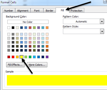
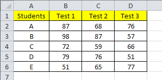
Click OK and you’ll now see that the color has been changed for the selected cells.

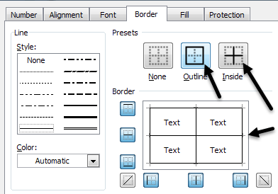
Let’s also add some borders between the cells so that if we decide to print out the Excel sheet, there will be black lines between everything. If you don’t add borders, the lines you see in Excel by default do not print out on paper. Select the entire grid and go to Format Cells again. This time go to the Border tab. Click on the Outside and Inside buttons and you should see the small display box directly below the buttons change accordingly with the borders.

Click OK and you should now have black lines between all of the cells. So now we’ve formatted our grid to look much nicer! You can do this type of formatting for your data also in the way you feel appropriate.

Using Formulas and Functions in Excel

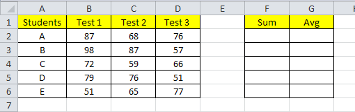
Now let’s get to the fun part: using Excel functions and formulas to actually do something! So we want to first calculate the average grade for our 5 students after their 1st three exams. Excel has an average function that we can use to calculate this value automatically, but we’re going to do it slightly differently in order to demonstrate formulas and functions.
Add a header called Sum in column F and Avg in column G and format them the same way we did the other header cells.

Now first we’ll use Excel’s sum function to calculate the sum of the three grades for each student. Click in cell F2 and type in “=sum(” without the quotes. The = sign tells Excel that we plan on putting some type of formula into this cell. When you type in the first parenthesis, Excel will display a little label showing you what types of variables this function takes.

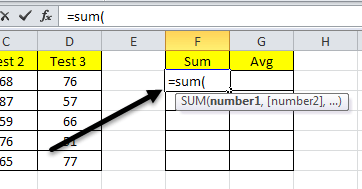
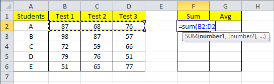
The word SUM is a built-in function in Excel which calculates the sum of a specified range of cells. At this point after the first parenthesis, you can select the range of cells you want to sum up! No need to type the cells one by one! Go ahead and select cells B2 to D2 and you will see that the formula is automatically updated and is in blue.

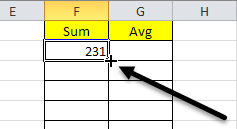
After you select the range, type in the closing parenthesis (Shift + 0) and press Enter. And now you have the sum of the numbers! Not too hard right!? However, you might say that it would be a royal pain to do this for a set of 100 or 500 students! Well, there’s an easy way to copy your formula automatically for the other students.
Click on cell F2 and then move your mouse slowly to the lower right edge of the cell. You’ll notice that the cursor changes from a fat white cross to a skinny black cross and the bottom right of the cell is a small black box.

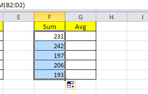
Click and hold your mouse down when it changes and then drag it to the row of the last student. And with that, Excel uses the same formula, but updates the current row cells so that the sum is calculated for each row using that row’s data.

Next, click in cell G2 and type the = signs to denote we are starting a formula. Since we want to divide the sum by 3 to get the average, type the = sign and then choose the sum cell F2. Continue on with the formula by typing in “/3”, which means divide by 3.

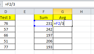
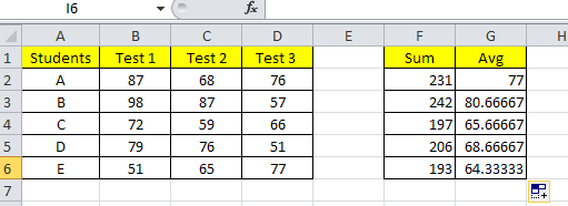
Press Enter and you now have entered your own average forumla! You can use parenthesis and perform all the math functions in this same way. Now do the same thing as we did with the average column and click the small black box at the lower right corner in cell G2 and drag it down to the bottom. Excel will calculate the average for the rest of the cells using your formula.

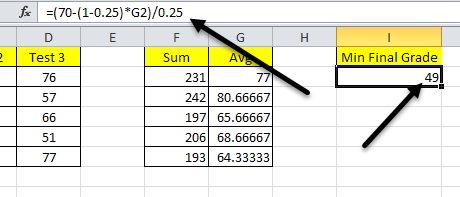
And lastly, let’s put in one more formula to calculate what each student would have to get on the final in order to get an A in the class! We have to know three pieces of information: their current grade, the passing grade for the class and what percent the final is worth of the total grade. We already have their current grade which we calculated and we can assume a 70 is the passing grade and the final is worth 25% of the total grade. Here is the formula, which I got from this site.
Final Grade = Exam Worth x Exam Score + (1 – Exam Worth) x Current Grade
Final Grade would be the 70 since that is the passing score we are assuming, Exam Worth is .25 and we have to solve for Exam Score. So the equation would become:
Exam Score = (Final Grade – (1 – Exam Worth) x Current Grade)/ Exam Worth
So let’s create a new header in column I and in cell I2, beging typing “=(70-(1-.25)*” and then select cell G2 and then continue on with “)/.25” and then press Enter. You should now see the grade required and also the formula in the formula bar above the column names. As you can see below, Student A needs to get at least a 49 to make sure they get a 70 passing score for their final grade.

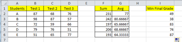
Again, grab the bottom black box of the cell and drag it down to the bottom of the data set. And viola! You’ve now used Excel functions, created your own formulas in Excel and formatted cells to make them visually appealing.